Alternate Shading

If you find that your data moves around a lot and you would like to apply automatic alternate shading to a range of cells then this is possible using Conditional Formatting.

Select the cells you want to shade and select (Format > Conditional Formatting).
For more information about Conditional Formatting, please refer to the Conditional Formatting section.
You can use formulas to determine the outcome and depending on the formula used it does not even have to contain any cell references.
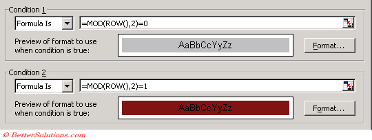
In Condition 1 type the following formula "=MOD(ROW(),2)=0".
The ROW function returns the row number of the current cell and then the MOD function is used to obtain the remainder after dividing this number by 2. This formula is True for any cells that have even row numbers.
In Condition 2 type a similar formula "=MOD(ROW(),2)=1".
This formula is True for any cells that have odd row numbers.

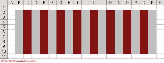
Shading alternate Columns

You can use an identical method to the one above to apply automatic shading to your columns as well.
In Condition 1 type the following formula "=MOD(COLUMN(),2)=0".
In Condition 2 type the following formula "=MOD(COLUMN(),2)=1".

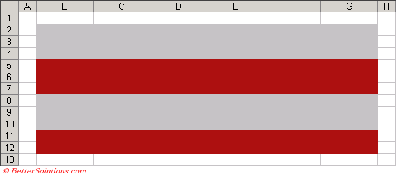
Shading alternate Rows (Bands)

You can use a similar method to the one above to apply automatic shading to bands of rows.
In this example we want to shade the rows in blocks of 3.
In Condition 1 type the following formula "=MOD(ROW()-2,3*2)+1<=3".
In Condition 2 type the following formula "=MOD(ROW()-2,3*2)+1>3".

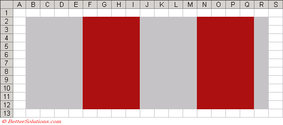
Shading alternate Columns (Bands)

You can use a similar method to the one above to apply automatic shading to bands of columns.
In this example we want to shade the columns in blocks of 4.
In Condition 1 type the following formula "=MOD(COLUMN()-2,4*2)+1<=4".
In Condition 2 type the following formula "=MOD(COLUMN()-2,4*2)+1>4".