Creating

There are several advantages when you convert a regular list to an actual List Object
New rows and columns are automatically included.
A total row at the bottom of your list can be easily added to display sums, averages, counts etc.
You can easily print the whole list.
Columns added to the right are automatically incorporated into the List object.
Charts based on rows and columns will be expanded automatically.
Named Ranges assigned to rows and columns will be expanded automatically.
The list is protected from accidental row and column deletion.
This list can be published to a SharePoint site.

Creating a List Object

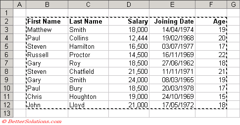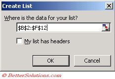
Select any cell within your list and select (Data > List > Create List)
This will display the Create List dialog box.

Adding new rows and columns

Toggle Total Row

(Data > List > Total Row)
Excel inserts a new row at the bottom of your list and automatically displays the sum of the last column.

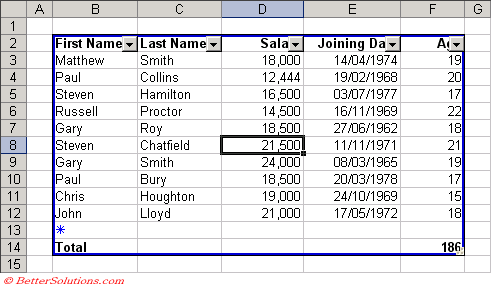When you select the last cell of any row an additional drop-down list appears allowing you to select from any of the aggregation functions.
The total row uses the SUBTOTAL function to perform the necessary aggregation.
These total rows only reflect the rows that are currently visible, any hidden rows causing by filtering are ignored.

By selecting one cell in the data Excel 2007 automatically select the current region of cells that contain data.
However you can select a different range of cells to use when creating a table if you want.
In addition if your data does not contain headers, Excel 2007 creates them for you and labels them as Column1, Column2 etc

Format as Table dialog box

Excel 2007 converts the data in the workbook into a table
Each column header contains an Autofilter arrow and a black border surrounding the data, which means that the table is active on the worksheet.

The table must be active on the worksheet for the Design contextual tab to appear.
To make a table active click in any cell.

The tables feature (formerly Lists in Excel 2003)
When you open a 2007 workbook that contains a Table in Excel 2003 the table will appear but none of the surrounding functionality will be available.
This means the table can be modified and the table should remain intact when re-opened in Excel 2007.
However any structural changes made to the workbook such as inserting or deleting cells and columns may cause the table - not the data to be lost when the file is re-opened in Excel 2007.

Many of the new enhancements to Tables in Excel 2007 will mean that tables will not be recognised as Lists when opened in previous versions of Excel.
For example when the header row of the table is disabled, when the total row contains text or custom formulas that were previously not available
In these cases you will still be able see and edit the data but the list properties will not be there.

Selecting Tables

Inserting Data

Just type and press Tab
Right mouse click and use Pick from List

Table Columns to the Left

Table Rows Above

Inserting Data from Pictures

link - support.microsoft.com/en-gb/office/insert-data-from-picture-3c1bb58d-2c59-4bc0-b04a-a671a6868fd7

Total Row

changing to average and count
add to another column by just clicking in cell and using drop-down

create a table and add a SUM formula below

Options

Header Row

Banded

First and Last

Copying

Copying the Results to Another Location

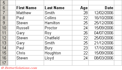
Instead of filtering the list in-place you could copy the results to another location on the same worksheet.
It is not possible to copy the results to another worksheet or workbook.
The criteria can be on a different worksheet but the results can only be copied to the same worksheet.

More Complicated Formulas

The example we are going to use here will use a more complicated formula in its criteria.
When you use more complicated formulas the criteria heading used must not be the same as any of the table column headings.
In this case we have used the heading "Criteria" instead of "First Name".
If you use the heading "First Name" only the heading appears in the "Copy to location".
Alternatively you could leave it blank but even when left blank the criteria still needs to include both cells.

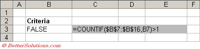Any formulas you do use have to return either TRUE or FALSE.
You will also need to include the necessary absolute and relative references (in this case cell "B7").
A particular row is only included when the formula returns TRUE for that particular line.

Creating the Formula

In this example we are going to extract all the names that appear more than once in the "First Name" column.
The function that can help us with this task is the COUNTIF function.
This function returns the number of cells with a value that satisfies a condition.

Absolute and Relative References

When you are using formulas for your conditions it is important to know when to use absolute and when to use relative references.
Absolute references should be used for any cell ranges that you want to remain fixed within the formula.
Relative references should be used for any cell ranges that are relative to the row that is being analysed at the time.
For example we want to be able to determine if an item appears more than once in a particular column.
For this we will use an absolute cell reference for "B7:E16" but a relative cell reference for the cell range passed as the criteria to the COUNTIF function.

Enter the Condition

Enter the following formula in cell "B3" above the table.

Select a cell inside the table, for example cell "C7" and select (Data > Filter > Advanced Filter).
Check that the "List range" references the whole table.
In the "Criteria range" textbox select the cells "B2:B3".
Select the option "Copy to another location".
In the "Copy to" textbox select cell "B18" (this is the first cell where you want the results to start).
Check you have entered all the information correctly and press OK.

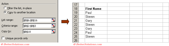Extract - Worksheet Level Named Range

When you specify a "Copy To" range Excel will automatically assign the named range "Extract" to the "Copy To" cell range.
This named range can be used to quickly select the extacted range.
Select (Edit > GoTo) and type in "Extract" and press OK.
This probably wont be much use though because in this case it only refers to the first cell, i.e. cell "B18".

Remember

Criteria on the same line (different columns) are joined by AND and criteria on a new line (same column) are joined by "OR".
You can quickly display all the rows from a filtered list by selecting (Data > Filter > Show All).