Text

Understanding the Format

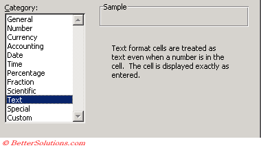To convert cells containing numbers to text, apply the Text format then press F2 to re-enter the data.

Editing Text

You can quickly move between words in a cell by holding down the Ctrl key and pressing with the left or right mouse button.

Replacing Text

The easiest way to replace text in your cells is to use the (Edit > Find) dialog box.

Useful Characters

CHAR(42) = comma
CHAR(32) = space
CHAR(10) =

Remember

When you enter text into a cell, if the contents will automatically spill over to the next adjacent cell assuming that the cell is empty. If the cell is not empty then the text will be truncated to the width of the column.
In Excel 2002 any numbers which are preceded with an apostrophe will have a Smart Tag attached to them. This will allow you convert the 'text' value to an actual number if you want.
Text entered into a cell is often referred to as a 'string'. It may also be referred to as a 'text string'.
Each uppercase character is exactly 32 characters lower than its corresponding lowercase characeter.

Entering Text

By default text is aligned and numbers are right aligned.
A cell can hold up to 32,000 characters of text although it is not recommended to have more than 255.
Not all the text functions will return the correct answer when a string contains more than 255 characters.
With text wrap formatting set in a cell (Format > Cells)(Alignment tab, Wrap Text), sometimes you want to force a line break at a certain point. You can use (Alt + Enter)
SS

You can enter tabs and carriage returns in a cell to make the text easier to read.
To enter a tab, press (Ctrl + Alt + Tab).
To enter a carriage return press (Alt + Enter).
Carriage retursn cause the contents of the cell to wrap within the cell.

Numbers as Text

When you enter a number into a cell it is automatically right aligned.
When you enter text into a cell it is automatically left aligned.
There may be times when you have entered a number but you want it to be considered as text.
There are two ways you can achieve this:
1) Select (Format> Cells)(Number tab) and select the Text category.
2) Place an apostrophe before the actual number. Don't worry this apostrophe is not displayed it just automatically formats the cell as Text.
Even though a cell is formatted as text it can still be used in 'some' functions and formulas.

SS A1 + 5 - when A1 is formatted as text
SS SUM() - does not work !!

Data (i.e. values) you import into Excel is often treated as Text. This can be quickly rectified by multiplying the data by 1.
SS - Example - how to multiply by 1

Concatenating Text

Excel uses the ampersand "&" character for string concatenation.
The concatenation is a word that means to join two strings together.
This can be used in formulas to combine the contents of multiple cells.
SS
There is also a CONCATENATE function.
You can add spaces by enclosed them in speech marks
SS
Alternatively you can use the CHAR(32) to represent a space
SS

Using TEXT to format values used in a text string

"The total sales last year was" & ""
"This page was printed on : " & ""
Todays date is :Text(NOW(), " "_ & and time & Text(now(), " ")

Comparing Text

Comparing text strings for equality can be done using the "=" operator but it is important to remember that this is not case sensitive
SS ("better solutions" = "Better Solutions" when is cells
If you want to perform a case-sensitive text comparison then use the EXACT function.
SS

Proportional and Non Proportional Fonts

If the default font is a non-proportional (fixed width) font, such as Courier, 8.43 characters of any type (numbers or letters) fit into a cell with a column width of 8.43 because all Courier characters are the same width.
If the font is a proportional font, such as Arial, 8.43 integers (numbers such as 0, 1, 2, and so on) fit into a cell with column width of 8.43.
This is because numbers are fixed-spaced with most proportional fonts.
However, because letters are not fixed-spaced with proportional fonts, more "i" characters fit and fewer "w" characters fit.
When you change the width of a column to a fractional number, the column width may be set to a different number depending on the font used in the Normal style.
For example, with a Normal style font of Arial, if you attempt to change the width of a column to 8.5, the column is set to 8.57 or 65 pixels.
This behavior occurs because of the translation of font characters to pixel units.
Fractional pixel units cannot be displayed; therefore, the column width rounds to the nearest number that results in a whole pixel unit.

Using the Format > Cells dialog box

Shows how the selected font will appear, formatted with the options you have designated.

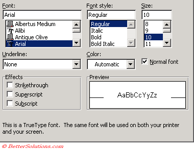Font - Select a font name to change the font of the selected text. Select the options you want on the Font tab to change the appearance of the selected text.
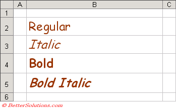
Font Style - Change the font style of the selected text.
In Excel 2007 font sizes can include 0.5pts - Is 6.2pts rounded down ??
Fonts are displayed in different sizes depending on the view % of the worksheet.
For example at 100% 11 and 11.5 look the same but at 110% they look different - SS

Size - Enter the font size for the selected text. You can type any number between 1 and 1638.
The sizes in the Size list depend on the selected font and active printer.
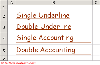
Underline - Select an underline type to format the selected text with an underline.

Color - Select a color from the list to change the color of the selected text or object.
If you select "Automatic" the colour will always be black ?
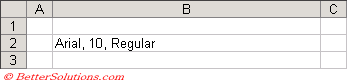
Normal font - You can change the text back to the default at any time.

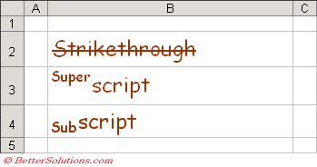
Strikethrough - Draws a line through the selected text.
Superscript - Formats the selected text or numbers as superscript.
Subscript - Formats the selected text or numbers as subscript.

Formatting Characters

When you select a cell or range of cells, any formatting is applied to the whole cell range and all of its contents.
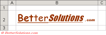
It is possible to apply formatting to individual characters within a cell.
To format characters within a cell, double click the cell with the left mouse button (to enter edit mode).
Highlight the characters you want to format. You will only be able to use the formatting options from the Font tab.

Text to Numbers

Sometimes numbers can look like numbers when they are infact text.
All numbers should be right aligned by default
If numbers are left aligned then they are probably being interpreted as text.
It is not possible to perform calculations on any numbers that are being interpreted (or formatted) as text

SS
Example SUM

This often happens when you import data from Access

Identifiying Numbers formatted as Text

(Tools > Options)(Error Checking tab, "Number stored as text")
Excel will frag any cells that contain numbers that are formatted as text
A green flag will be displayed in the top left corner click menu button and select "Convert to Number"

1) Multiple the values by 1 using Paste Special

Never Change the Alignment

If the alignment is not changed, then only numbers aligned on the right will be used in numerical calculations.
To avoid any unpredictable results in your formulas never manually change the alignment, this way you can easily spot any numerical values that are being interpreted as text.
If you want to have a currency symbol appear before a numerical value then you need to apply the relevant number format.

Multiply by 1

When you copy or import data from other applications the numbers are often inserted as text.
All the values in column B are being treated as text. You know this from their alignment.
Text is always aligned on the left. Numerical values are always aligned on the right when using the "General" number format.

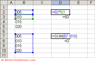The formula is cell D2 refers to cells B2 and B3 and returns the correct result, which is 50.
However the formula in cell D7 which uses the SUM() function and refers to the range of cells "B7:B10" does not return the correct result.
You can easily convert the values in column B to actual numbers by multiplying them by 1. See screen shot below.
Enter the number 1 in cell D10. This can actually be placed in any cell.
Select cell D10 and press (Edit > Copy).
Select the range of cells containing the values (in this case "B2:B10") and select (Edit > Paste Special).
Choose the Multiply option button and press OK. This will multiply whatever is on the clipboard (in this case the value 1) to the highlighted range.

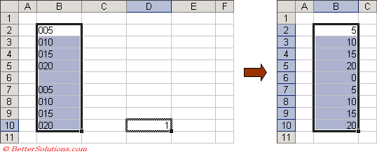Once the values have been converted to numbers all worksheet functions will return the correct results.
You can also convert text values to numerical values by using the Text Import Wizard. For more details please refer to the Text To Columns page.

Remember

You can toggle bold on the current selection by using the shortcut key (Ctrl + B).
You can toggle italics on the current selection by using the shortcut key (Ctrl + I).
You can toggle underlining on the current selection by using the shortcut key (Ctrl + U).
You can toggle the strikethrough of text on the current selection by using the shortcut key (Ctrl + 5).
A quick way to remove the formatting attached to a cell is to select (Edit > Clear > Formats > Clear).