Getting Started

It is possible to run, record and share your scripts with other workbooks and colleagues using the Automate Tab.
This tool is extremely useful regardless of how much programming experience you have.
At the moment the Automate tab is only available in Excel.
There is no Automate tab in Word, PowerPoint or Outlook. These applications do not currently support Office Scripts.
Office Scripts was specifically designed for Excel and is tightly coupled to the workbook and worksheet object models.

Lots of Samples

Before we run any samples, create a New Blank workbook and remove all the sheets except Sheet1.
Display the Automate tab and select (View Scripts > Samples).
The Office Scripts task pane will be displayed showing a list of all the sample scripts.
In the top right corner there are two different views: expanded view and compact view.
Here is the compact view.

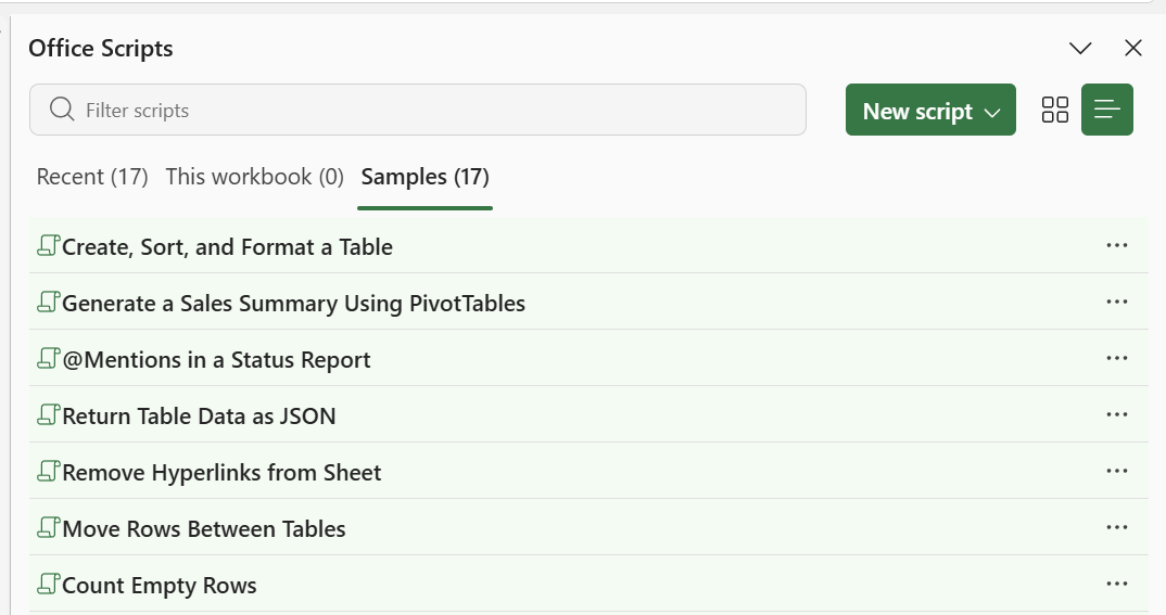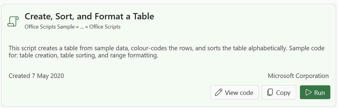
Find the sample "Create, Sort, and Format a Table".
Switch the view to expanded view and press the "Run" button to execute this script.

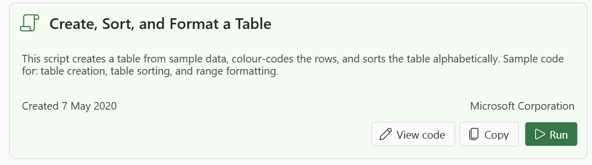This script creates a blank workbook and inserts sample data into cells "A1:C5".
It applies colour formatting, defines the cell range as a table and then sorts the table by the first column.
Press the "View code" button to display this script.

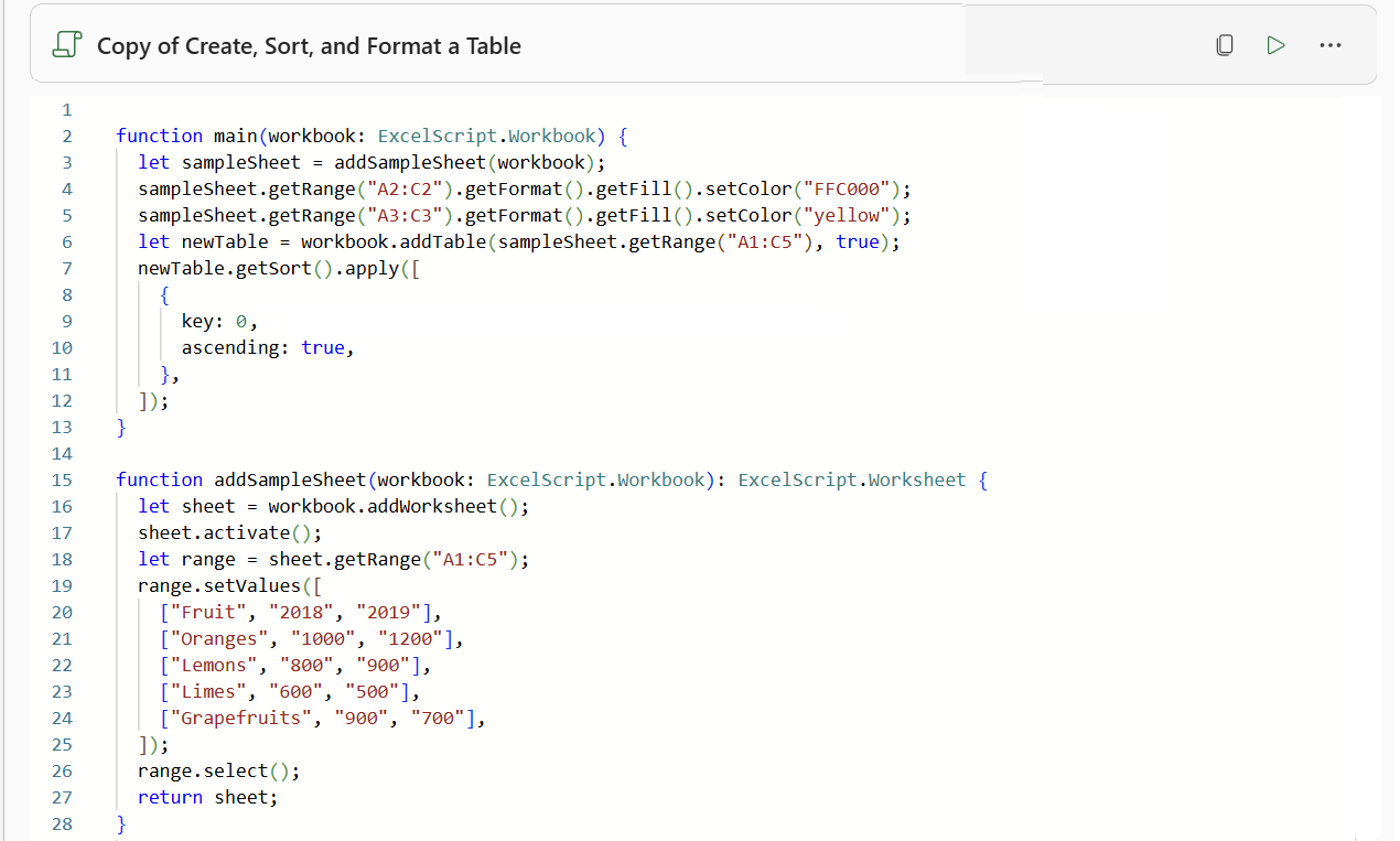This code is actually TypeScript, which is a superset of JavaScript.
This script contains two functions:
main - This is the starting point for all office scripts.
addSampleSheet - This is a helper function that is called from the main function.
All office scripts need to have a main function that accepts an argument of type ExcelScript.Workbook.

Understanding the Script

Here is a description of what actually happens when this script runs.
The first thing this script does is insert a new worksheet into the existing workbook.

let sheet = workbook.addWorksheet()

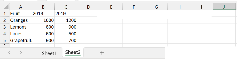
The cell range "A1:C5" is populated with the sample data.

let range = sheet.getRange("A1:C5"); 
range.setValues( [] );

The cell range "A2:C2" is shaded orange.

sampleSheet.getRange("A2:C2").getFormat().getFill().setColor("FFC000");

The cell range "A3:C3" is shaded yellow.

sampleSheet.getRange("A3:C3").getFormat().getFill().setColor("yellow");

The cell range "A1:C5" is converted to a table.

let newTable = workbook.addTable(sampleSheet.getRange("A1:C5"), true);

The table is then sorted, based on the first column. This is indicated by the key = 0.

newTable.getSort().apply([ 
  { 
    key: 0, 
    ascending: true, 
  }, 
]);

Saving a Copy

It is not possible to edit or change any of the sample scripts so lets make a copy.
Press the "Copy" button to create a copy of this script.

This will display the "Save a Copy" dialog box.
There are lots of different places you could save this script but for now, lets save it in the default Office Scripts folder.
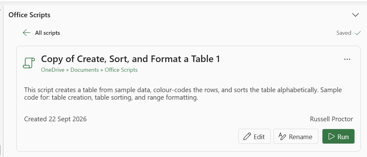
Once the script has been saved this will be indicated in the Office Scripts task pane.
Press the "Rename" button.

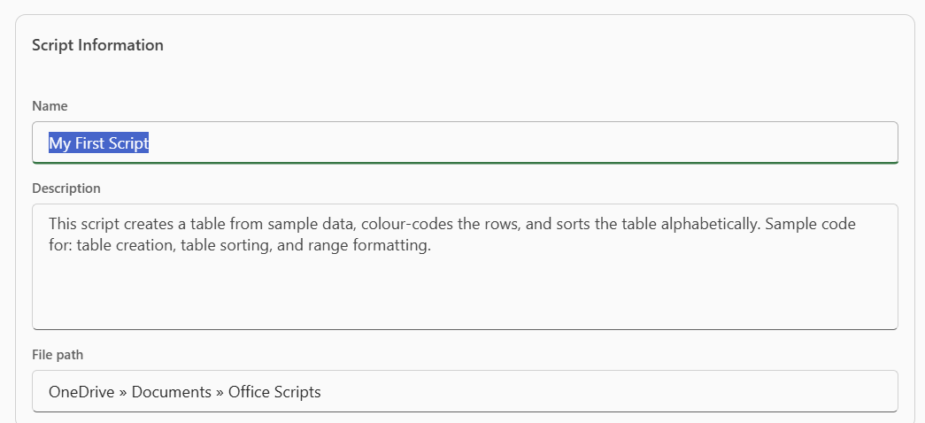
Enter a new name for this script in the Name box. Lets call it "My First Script".
The description can stay the same.
This screen also shows you the file path of where the script has been saved.

Editing the Code

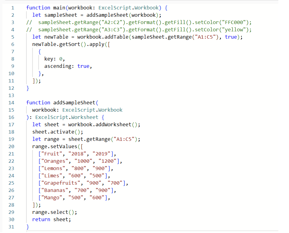
Press the "Edit" button to display the Code Editor.
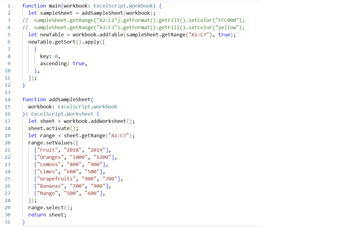
Lets add two more rows to the sample data and remove the colour formatting.
Row 3 - comment this out
Row 4 - comment this out
Row 26 - add Bananas, 700, 900

["Bananas", "700", "900"],

Row 27 - add Mango, 500, 600

["Mango", "500", "600"],

We also need to change the cell range.
Row 5 - change the cell reference to "A1:C7"
Row 19 - change the cell reference to "A1:C7"

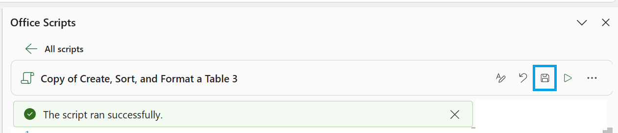
Press the "Save script" button to save your changes.

Then press the "Run" button to run the script again.
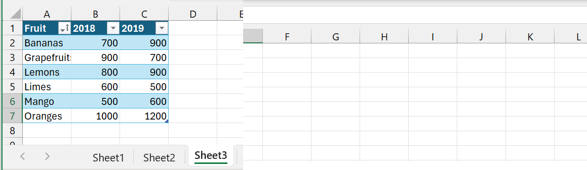
Once the script has run successfully you will see a message displayed at the top.
This is how the table looks after running our modified script.

If you run the script multiple times you will see a message asking if you want to add the script to the workbook.
Close the task pane.

Recording a Script

We can use the Action Recorder to record your actions and then replay it back at a later date.
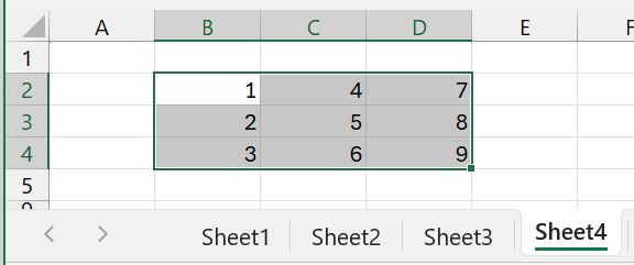
Insert a new worksheet into our workbook called "Sheet4".
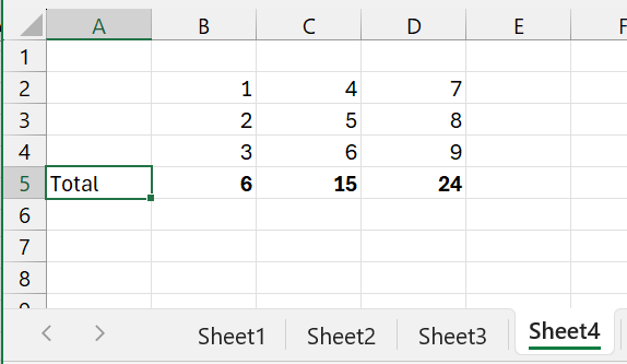
Enter some numbers into cell range "B2:D4".
What we would like to do is to add a total row underneath the table and apply bold formatting to this total.

To start recording select (New Script > Create from Recording).
Select "B5" and enter this formula.

=SUM(B2:B4)"

Drag this formula across to cells "C5" and "D5".
Apply bold to these 3 cells and add the word "Total" in cell "A5".

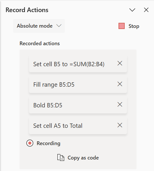
While you are recording your steps the task pane will update automatically with a short description.
A list of all the individual actions is displayed for reference.

Press the "Stop" button when you have finished all these steps.
Once the action recorder has been stopped the task pane will display a summary screen.

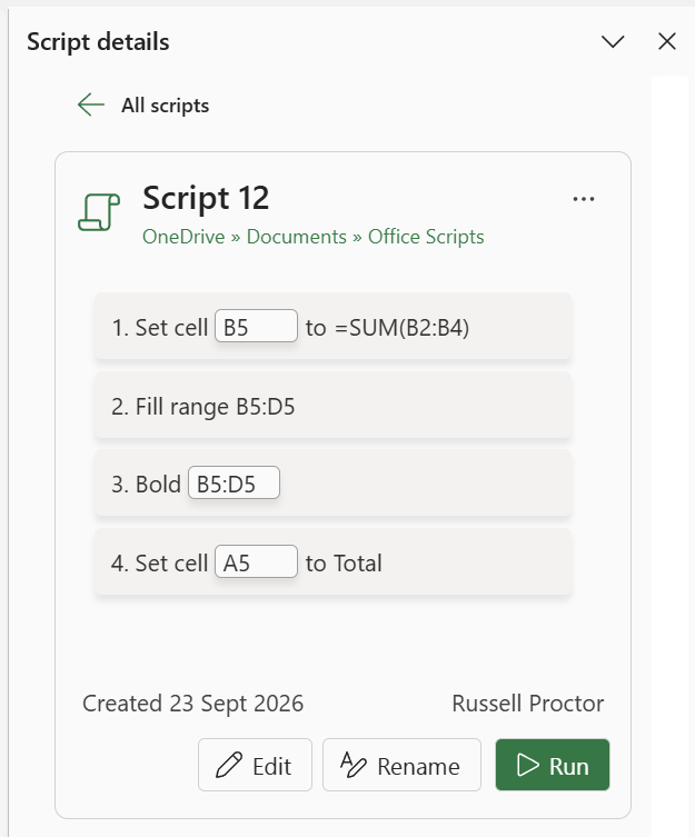Excel will automatically give your script a name ("Script 1", "Script 2", etc).
Change the name to "My Second Script" and select Rename.
Press the "Edit" button to see the script that has been recorded.

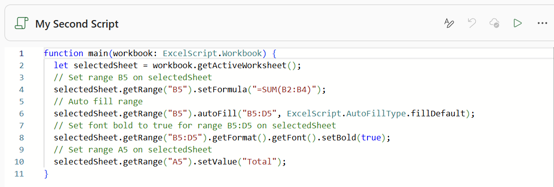You will see that every line of code has a comment above it.
Here is a description of what actually happens when this script runs.
Obtain a reference to the active worksheet.

let selectedSheet = workbook.getActiveWorksheet();

The cell "B5" is populated with the formula to add up the 3 cells above it.

selectedSheet.getRange("B5").setFormula("=SUM(B2:B4)");

Drag cell "B5" across to cells "C5" and "D5".

selectedSheet.getRange("B5").autoFill("B5:D5", ExcelScript.AutoFillType.fillDefault);

Apply bold to these 3 cells.

selectedSheet.getRange("B5:D5").getFormat().getFont().setBold(true);

Add the word "Total" in cell "A5".

selectedSheet.getRange("A5").setValue("Total");

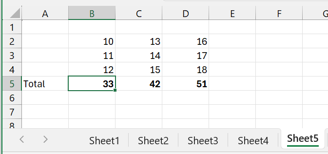
Lets test this script on a different data set.
Insert a new worksheet, called "Sheet 5" and enter some numbers into cell range "B2:D4".
Select cell "B5" and press "Run".

Enhancing the Script

This script works but it is not very useful in its current state.
For example the cell range has to be (3 x 3) and it also has to be in cells "B2:D4".
It would be great if the block of numbers could be anywhere on the worksheet and could be any size.
Lets go ahead and make these changes to the code.
Before we actually make any code changes we need to describe what we need to do.

Step 1 - Identify the top-left cell of the block of numbers. 
Step 2 - Work out how many rows there are in the block of numbers. 
Step 3 - Work out how many columns there are in the block of numbers. 
Step 4 - Calculate the row number for the cell containing the word "Total". 
Step 5 - Calculate the column number for the cell containing the word "Total".

We also need to write down any assumptions that we are making.

Assumption 1 - That one of the cells in the block of numbers is selected when we run the script. 
Assumption 2 - That the block of numbers is not starting in column "A".

Now that we have the list we can find the corresponding code for each step.

Step 1 - To get the current region we can use getSurroundingRegion and use the getCell method and pass in the top-left index position.

let selectedSheet = workbook.getActiveWorksheet(); 
let currentRegion = workbook.getActiveCell().getSurroundingRegion(); 
let topLeftCell = currentRegion.getCell(0, 0); 
let leftColumn = topLeftCell.getColumnIndex(); 
let topRow = topLeftCell.getRowIndex();

Step 2 - To get the number of rows in the block we can use getRowCount.

let numberOfRows = currentRegion.getRowCount();

Step 3 - To get the number of columns in the block we can use getColumnCount.

let numberOfColumns = currentRegion.getColumnCount();

Step 4 - To get the row number for the total we need to add the top-left row to the number of rows.

let totalRowNumber = topRow + numberOfRows;

Step 5 - To get the column number for the total we need to get the column letter from the top-left cell and minus 1.

let totalColumnNumber = leftColumn - 1;

With that additional information we are now in a position to be able to replace the following cell references.
Instead of cell "B5" we can use.

let firstTotalCell = selectedSheet.getCell(totalRowNumber , leftColumn);

Instead of "B2:B4" we can use.

let sumRange = selectedSheet.getRangeByIndexes(topRow, leftColumn, numberOfRows, 1);

Instead of "B5:D5" we can use.

let dragRange = selectedSheet.getRangeByIndexes(totalRowNumber, totalColumnNumber + 1, 1, numberOfColumns);

Instead of "A5" we can use.

let totalCell = selectedSheet.getCell(totalRowNumber , totalColumnNumber - 1);

Modified Script
We are now in a position to replace all the hard coded cell references with dynamic cell references.

firstTotalCell.setFormula("=SUM(" + sumRange.getAddress() + ")"); 
firstTotalCell.autoFill(dragRange, ExcelScript.AutoFillType.fillDefault); 
dragRange.getFormat().getFont().setBold(true); 
totalCell.setValue("Total");

Lets go ahead and replace our script and see if it works. Press the "Run" button.

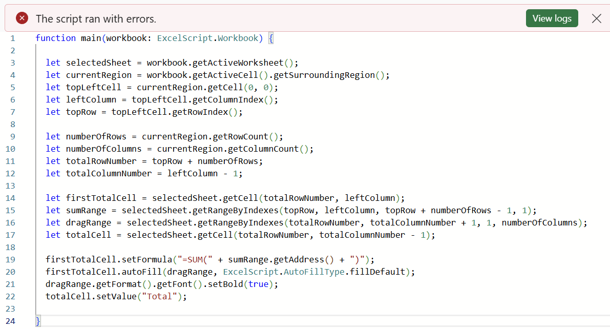If the script is unable to run the Output window will appear and a message will be displayed.

Line 17: Worksheet getCell: Parameter out of range

On line 17 we are subtracting 1 from the totalColumnNumber, but this is not necessary because 1 has already been subtracted on line 12.
We can change line 17 to this instead.

let totalCell = selectedSheet.getCell(totalRowNumber , totalColumnNumber);

Make this change and save the script.
Press the "Run" button to run the script again.
This time everything work and we get the right result.
Now lets increase the size of the block of numbers and also move it across and down the worksheet.
Enter some numbers into cell range "C4:F9" and test the script.
Close the task pane and close this workbook.

Creating a Script

We have looked at the samples and we have recorded our own steps. Lets now create a script entirely from scratch.
Create a New Blank workbook and remove all the sheets except Sheet1.
Select (New Script > Create in Code Editor).
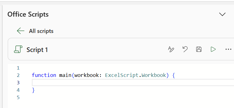
The Office Scripts task pane will open and some default code will be displayed.
Remove all the code inside the main function.

If you have found a script online that you want to use then you can just paste it straight in.
Copy the following script and paste it in to the code editor.

function main(workbook: ExcelScript.Workbook) { 
    // Insert a new worksheet 
    let selectedSheet = workbook.addWorksheet(); 

    // Create some sample data 
    let months = ["Jan", "Feb", "Mar", "Apr", "May", "Jun", "Jul", "Aug", "Sep", "Oct", "Nov", "Dec"]; 
    let mockData = months.map((month, i) => [month, Math.floor(Math.random() * 40) + 10 + i * 5]); 

    // Add headers and add the sample data block 
    selectedSheet.getRange("A1:B1").setValues([["Month", "Growth Metric"]]); 
    selectedSheet.getRange("A2:B13").setValues(mockData); 

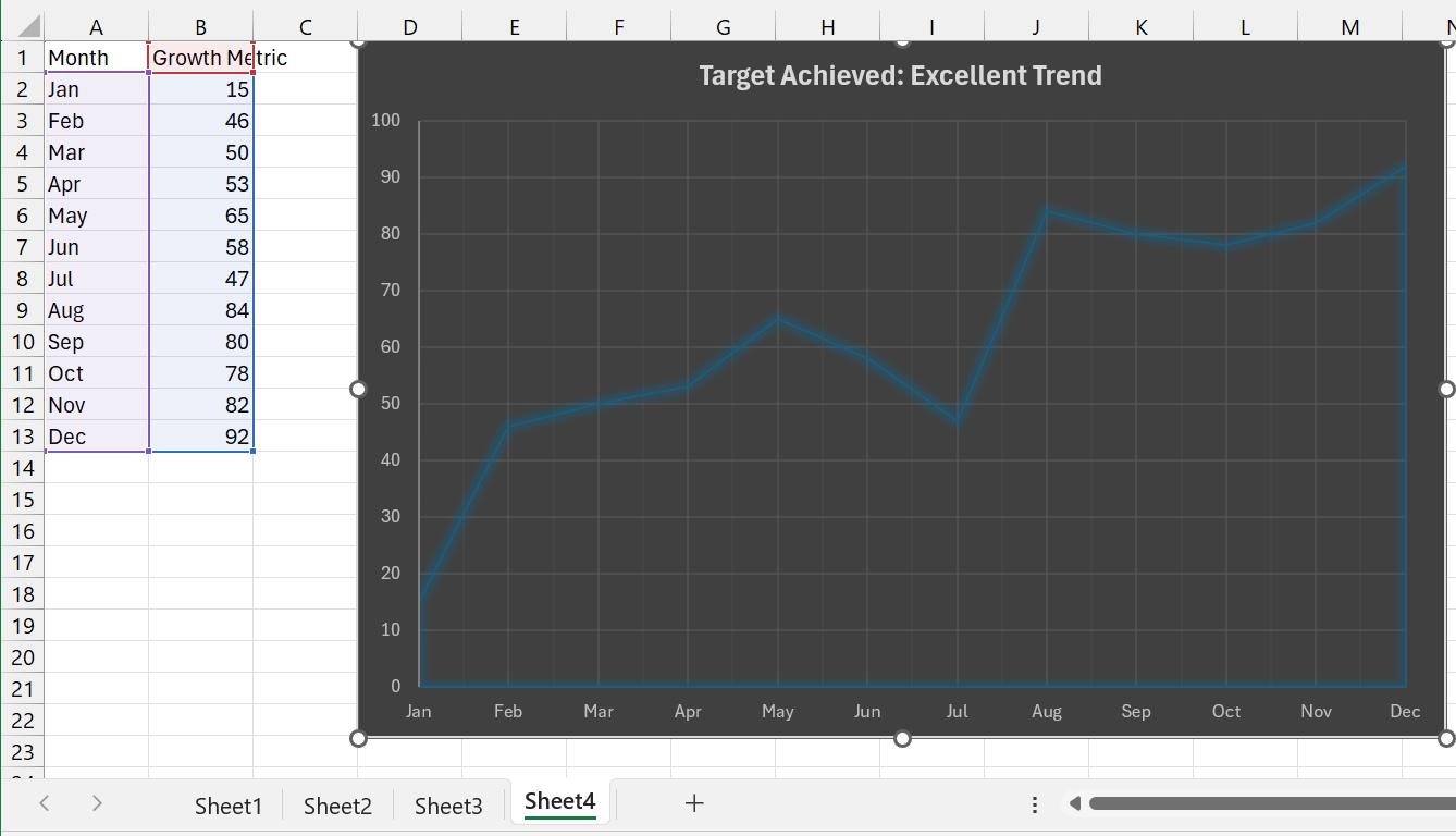
    // Create an area chart using the current region 
    let chart = selectedSheet.addChart(ExcelScript.ChartType.area, 
        selectedSheet.getRange("A1").getSurroundingRegion()); 
    chart.setPosition("D1"); 
    chart.setWidth(500); 
    chart.setHeight(320); 

    // Use a conditional statement to check if we reached our target 
    let finalPerformance = mockData[11][1] as number; 
    if (finalPerformance >= 60) { 
        chart.getTitle().setText("Target Achieved: Excellent Trend"); 
        chart.setStyle(245); 
    } else { 
        chart.getTitle().setText("Target Missed: Action Required"); 
        chart.setStyle(242); 
    } 
}

Run this script and check the results.
Run this script another two times and check that additional worksheets are added.

Notice that this script contains a conditional statement.
The action recorder cannot generate code that contains conditional statements or loops.

More Information

Buttons can be added to worksheets to let users quickly run scripts without having to use the Automate tab. more info
You can quickly share scripts across workbooks and with coworkers. more info
There are a few user settings that you can change. more info
You can combine Office Scripts with Power Automate to streamline entire workflows. more info
It is not possible to add a shortcut key to run a script at the moment.