Sorting

This section covers sorting your data when it is not been inserted into table.
If your data has been defined as a Table please refer to Tables > Sorting.

You can use the buttons on the Home Tab, Editing group
Or the buttons on the Sort & Filter drop-down
Or the buttons on the Data tab.
These two buttons allow you to sort your table based on a single column into either ascending or descending order.
To sort a single column just select any cell within the column you want to sort. Press either the ascending or descending button.

	Ascending - Sorts the data alphabetically from 1 to 100, A to Z, Jan to Dec and numerically from the lowest number to the highest. This is the default.
	Descending - Sorts the data alphabetically from 100 to 1, Z to A, Dec to Jan and numerically from the highest number to the lowest.

When you want to sort a table of data, there is no need to highlight the whole table first as the current region is automatically assumed when you only have a single cell selected.
Excel assumes that the list of data you want to sort is in a contiguous block separated by at least blank row and column.
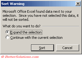
If you have highlighted only a selection within a contiguous block then Excel will warn you that you might not have the entire list selected and asks to confirm. The following dialog box is displayed.

Using the (Data > Sort) dialog box

Using the (Data > Sort) dialog box allows you to sort on as many as three columns at once.
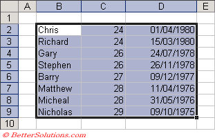
If you have a table of data you want to sort there is no need to highlight the whole table before pressing (Data > Sort) as the current region will be selected for you automatically.
Data is sorted in the following order: - Numbers, Text, Logical values, Error values, Blank cells.
Select any cell in the range "B2:C9" and when you select (Sort > Data) the whole current region will be selected automatically.

Your table of data may or may not contain a header row. A header row is the first row at the top of your table containing heading labels for each of the columns.
Assuming your table does not contain a header row the column letters are displayed in the drop-down boxes to allow you to identify the columns you want to sort.
The column containing the active cell is assumed to be the column you want to sort by first and will appear selected by default.

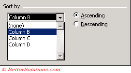Select the column letters in the order you want to sort the columns and then choose whether to sort the column into ascending or descending order.
If you have sorted that particular table of data before then the dialog box will display the parameters you last used.
You can easily undo the sort operation afterwards if you do not like the results by selecting (Edit > Undo) or pressing the Undo button on the Standard toolbar.

Using a Header Row

You table of data can contain a header row that can stay in place while all the other rows are sorted.

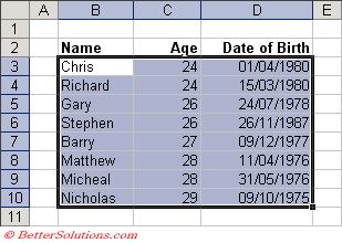When your table of data contains a header row the actual headings will be displayed in the drop-down boxes and not the column letters.
The column containing the active cell is assumed to be the column you want to sort by first and will appear selected by default.

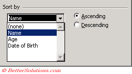Excel can normally recognise if your table of data contains a heading row or not and will change the option button accordingly.
You can change whether to include a heading row or not with the two option buttons at the bottom of the dialog box.

This is normally worth checking before you sort the data. If you accidentally sort the heading row you can just press (Edit > Undo).

Sorting cells with Formulas

It is possible to sort cells that contain formulas although be aware that some relative references will become invalid.
If you are sorting from top to bottom (i.e. rows) then any references to other cells in the same row will be unaffected.
Any references to other cells in different rows will become invalid.
The same is true when sorting by column, any references to other cells in different columns will become invalid.
you can avoid this potential problem by making sure that any cells referenced outside the table use absolute references or named ranges.
If your table of data is not too large, manually moving the rows or columns will maintain the correct references.

Sorting a single column

When you perform a sort on a single column of cells there is a chance that the continuity across the table may be broken.
Excel will now always prompt you to confirm the selection made when you try to sort a single column of data.
This gives you option of automatically expanding the selection to include the other columns in the table.

Sorting more than 3 columns

It is possible to sort on more than 3 columns if you need to.
You just need to sort the columns starting with the least important one first and finishing with the most important one.

Automatic Header Row

When you have text column labels and numerical values below Excel will automatically recognise the first row as a header row.
When you sort your list the header row will stay in place.

Remember

When you want to sort a table of data you do not need to select the table first as the current region will automatically be used or selected for you.
Excel will always sort the data based on the actual contents of the cell and not on the value that is displayed. This can be important if you are sorting dates.
It is possible to only sort on part of a list as long as you select the cell range first. This applies to using the buttons on the standard toolbar as well as the (Data > Sort) dialog box.
If you are trying to reduce the size of your toolbars you can remove the descending sort button from the Standard toolbar. The next time you want to sort a column in descending order hold down the Shift key while pressing the ascending order button.
Excel sorts objects, along with data as long as each object is contained within a single row or column.
Excel sorts the FALSE logical value before TRUE.
Any blank cells are always placed at the bottom of an Ascending Order list except when formulas return empty strings. When sorting these cells they appear below the numbers but before the text.

Custom Sorting

It is possible to create custom sort orders to sort your lists.
This is a great feature when you want to sort your list by something other than alphabetically or numerically.
Custom sorts and Custom lists are very closely linked.
If you are not familiar with Custom lists then you should read the page on Custom Lists first.

Using the Normal Sort

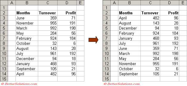
For example if your table contains a list of months you might want to sort it based on the logical order of those months.
Using the regular (Data > Sort) will sort this list into alphabetical order which is not that helpful.

Using a Custom Sort

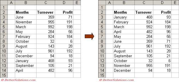
If you want the months to appear in their logical order then you can use one of the built-in custom sorts.
Select (Data > Sort) and enter the necessary sort by column.
Select the Options button in the bottom left corner to display the Sort Options dialog box.
This dialog box gives you a few extra options including which list to use for your sort.
In this example we want to sort the months so we choose the appropriate built-in custom list.
Press OK to close the Sort Options dialog box and then OK again to close the Sort dialog box.

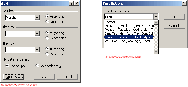The Sort Options dialog box will display all your custom lists in the First key sort order drop-down box.

Using Custom Sorting

Any custom sort is only applied to the first sort by field.
The ascending or descending option is ignored for a custom sort.
You cannot sort by more than one custom sort.
A custom sort sorts the items that match first and then the remaining items in ascending order underneath.

Case Sensitive

By default built-in sorts are not case sensitive.
If you want to perform a case sensitive sort you can use the Options dialog box and select the case sensitive option.

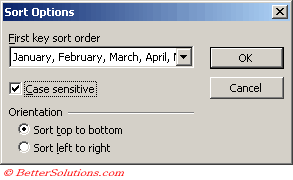First key sort order - Any custom lists that you have declared will be displayed in the drop-down list ?? Four custom lists are provided by default.
Case Sensitive - When Excel normally sorts data the case is irrelevant and "A" is the same as "a". This option allows you to sort by the uppercase letters first and then the lower case letters. This is not available when you sort items in a PivotTable report.
Sort top to bottom - This is the default. The columns remain in the same order and the rows are rearranged.
Sort left to right - This sorts your table of data by columns and not by rows. The rows remain in the same order and the columns are rearranged. The drop-down boxes will always display the row numbers as row headings are not recognised.

Using Conditional Formatting

If you want to sort a table of data based on the formatting applied by conditional formatting this is slightly more complicated.
For more details please refer to the Sorting By Conditional Formatting page.

Sorting By Colour

There is no built-in way to sort your cells (or rows) using their colour formatting.
However it is possible by inserting an extra column and then using a user defined function.
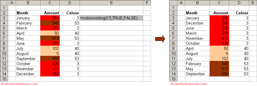
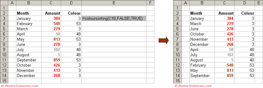
The user defined function will return a number indicating the colour of the cell used in that particular cell (or row).
You can then use the normal (Data > Sort) command using this new column as your first sorting column.

Additional Column

Lets assume that you have a simple table of data and that the formatting has been applied manually (NOT using Conditional Formatting).
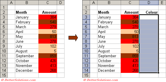
You must first add another column to your table of data.
This extra column will contain a user defined function which can be used to indicate the order in which to sort the rows.

Manual Formatting

The "manual" formatting you can use on cells is quite limited and you can only choose from the 52 colours on the colour palette.
You can either change the background colour or you can change the colour of the text.
If you want to sort using the background colour of the cells you can refer to the Interior property of the Range object.

Range("C3").Interior.ColorIndex 

If you want to sort using the colour of the text you can use the Font property of the Range object.

Range("C3").Font.ColorIndex 

User Defined Function

This user defined function will return the colour index of the cell reference which is passed as the first argument.
The number returned will always be between 1 and 52 since this corresponds to the location on the colour palette.
Once the user defined function has been entered into a code module in the corresponding VBA Project you can use it in your extra column.
If the cell does not contain any manual formatting then 0 is returned.

Option Explicit 

Public Function ColourSorting(ByVal rgeCell As Range, _ 
                              ByVal bBackGround As Boolean, _ 
                              ByVal bText As Boolean) As Integer 

   If bBackGround = True Then ColourSorting = rgeCell.Interior.ColorIndex 
   If bText = True Then ColourSorting = rgeCell.Font.ColorIndex 
   If ColourSorting < 1 Then ColourSorting = 0 
End Function 

Sorting by Background Colour

Sorting by Text Colour

Using Conditional Formatting

If you want to sort a table of data based on the formatting applied by conditional formatting this is slightly more complicated.
For more details please refer to the Sorting By Conditional Formatting page.